GridFlow Trade — AI-Powered BESS Trading Platform
Figures
 Open full size
 Open full size
 Open full size
 Open full size
 Open full size
Overview
A production ML system for GB day-ahead power prices and battery trading. It runs the whole loop in production: live ingestion, validation, training, a versioned registry, batch and API serving, data and drift monitoring, automatic rollback or gated retraining, and walk-forward backtesting of the trading strategy. It runs live at gridflowtrade.com with a public read-only demo, against a database that has been collecting since January 2023.
Problem
UK electricity prices are highly non-stationary — they are driven by renewable intermittency, demand cycles, interconnector flows, and system stress events. Naïve models trained on raw price series massively overfit to temporal leakage, producing misleadingly good in-sample results that fail out-of-sample.
The leakage, and what it cost
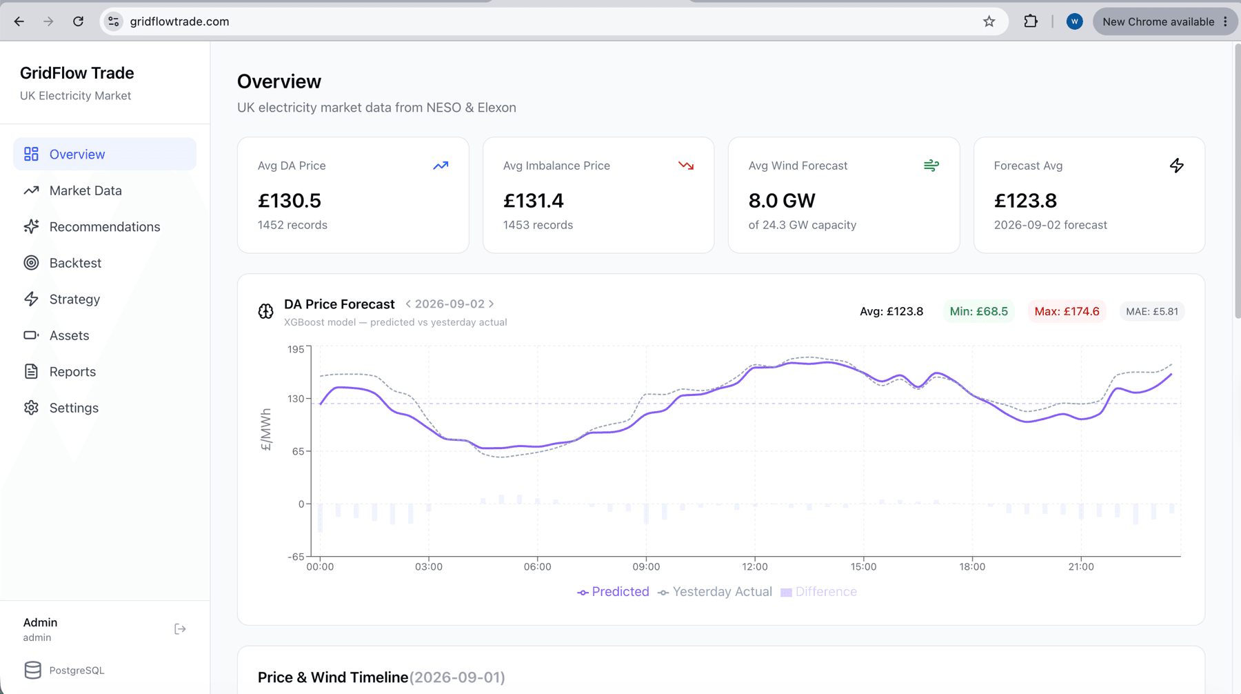
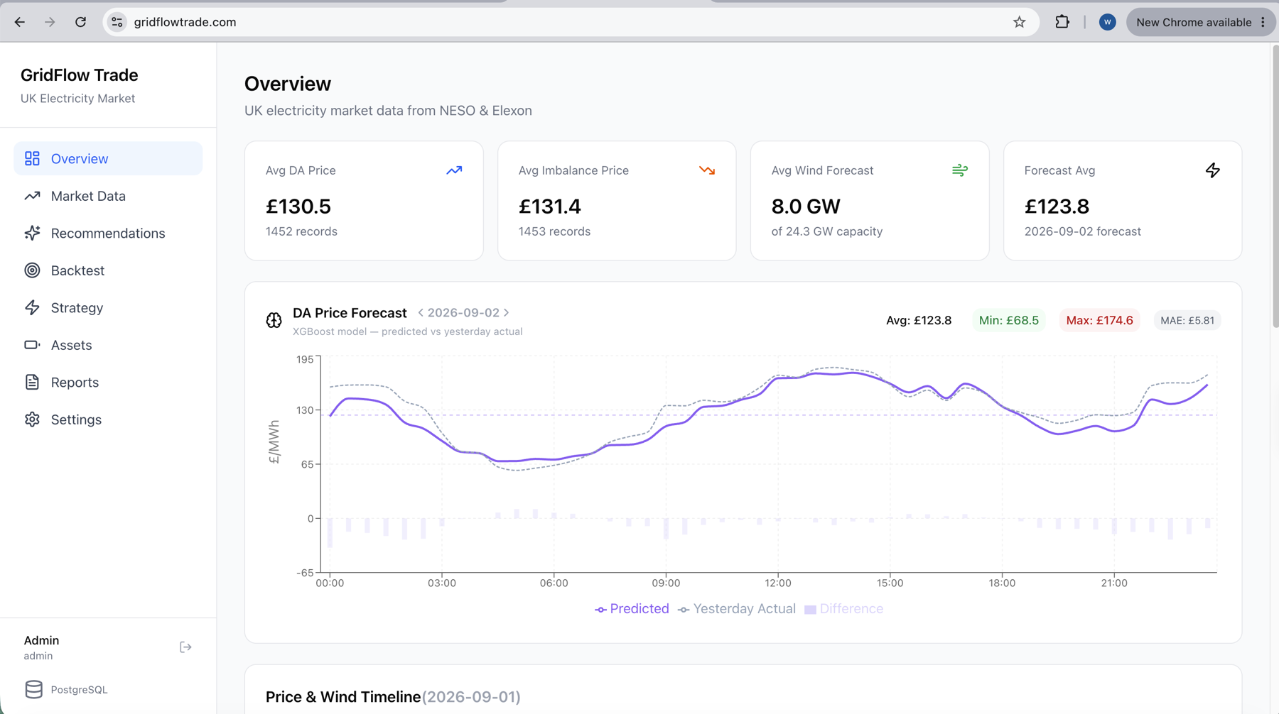
Early accuracy looked strong and was wrong. Training showed MAE £7.4 while the same model served in production sat at £21.9. The cause was target leakage plus train/serve skew: training and inference were not looking at the same features. The fix was a single point-in-time feature pipeline shared by both paths, fixed at the D-1 09:30 decision time so only data published by then can enter a forecast, with tests proving the two paths produce identical features and that future data cannot change a past forecast. The same pattern turned up twice more, in my own realised-accuracy monitoring and on the public dashboard, both of which were scoring forecasts cached after the day had already begun. That one mattered more than it looks: the automatic rollback rule reads that metric, so an optimistic number there could have stopped a rollback firing on a real degradation.
Model selection, and why it was not the interesting part
Naive, Ridge, LightGBM, XGBoost and a bidirectional LSTM were benchmarked on one leak-free split and tracked in MLflow. The tree models and Ridge were indistinguishable within seed noise, and the LSTM was worse. That is worth saying plainly: the gains came from feature design and evaluation design, not from choosing a better model. An ablation put the NESO day-ahead wind, demand and solar forecasts, collected at publication time so they are genuinely available before the auction, at 22% of the error reduction on their own.
Results
The reported accuracy was inflated by target leakage and train/serve skew: training showed MAE £7.4 while the same model served in production sat at £21.9. Rebuilding it as a single point-in-time feature pipeline shared by training and inference put the honest figure at MAE £24.2/MWh against a £34.2 naive baseline, a 29% error reduction on a 90-day held-out window averaged over five seeds. Benchmarking Naive, Ridge, LightGBM, XGBoost and a bidirectional LSTM on one leak-free split showed the tree models and Ridge were indistinguishable within seed noise, so the gains came from feature and evaluation design rather than model choice. Across a 12-month walk-forward with monthly refits, where every forecast is out of sample, it sits 23% below naive and is better in 11 of 12 months. GridFlow Trade was selected for the QMUL QIncubator programme and pitched to an investor panel in April 2026.
The data layer, which is most of the work
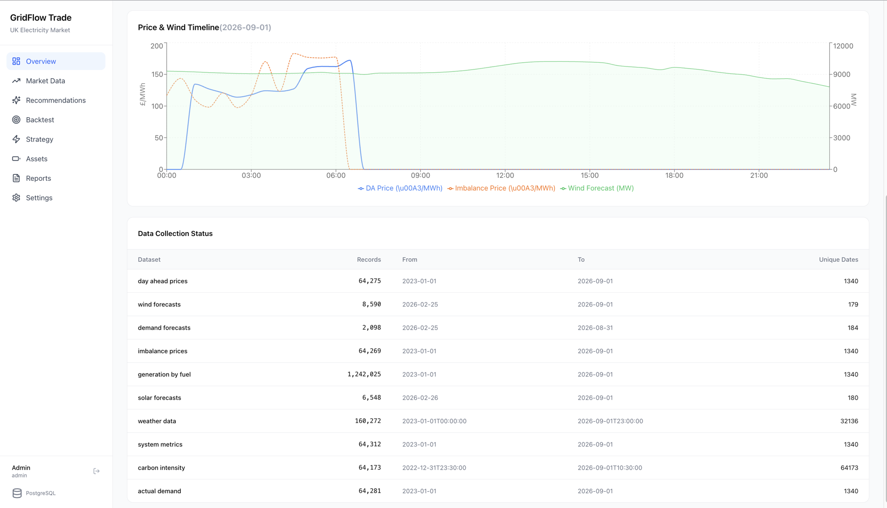
Ten datasets on a continuous collection schedule since January 2023 — roughly 1.7M rows in PostgreSQL. Day-ahead and imbalance prices, generation by fuel (1.24M rows on its own), wind and solar forecasts, demand forecasts and actual demand, weather, carbon intensity and system metrics, from NESO and Elexon. The collection-status view is part of the app rather than a separate dashboard: every dataset shows its row count, its coverage window and its number of distinct dates, so a feed that has quietly stopped is visible on the front page rather than discovered later. A price model trained across an unnoticed gap still produces a number, and the number still looks fine.
From a forecast to a schedule
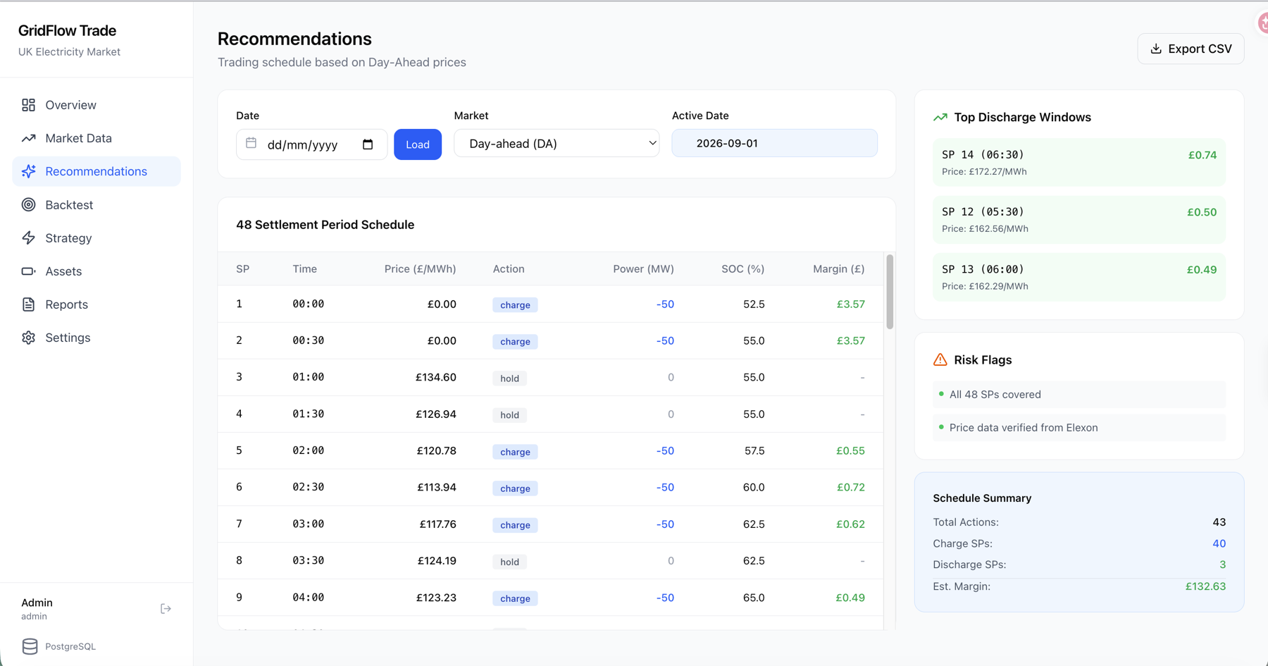
A price forecast is not a decision. The scheduler turns it into an action for each of the 48 half-hourly settlement periods in a UK trading day — charge, hold or discharge — subject to the battery's power rating and its state of charge, since you cannot discharge energy you have not stored and every charge decision constrains the ones after it. The output is the full 48-period table with the resulting SOC trajectory and margin, the best discharge windows, and a short set of checks: all 48 periods present, prices reconciled against Elexon. A schedule with a hole in it is worse than no schedule, because it looks complete.
What the strategy is actually worth
Forecast accuracy is not the thing anyone is buying. The backtest replays the linear-programming dispatch (SciPy HiGHS) at realised prices over 360 days and reports three numbers, because one of them alone means nothing: what the strategy made, what perfect foresight would have made, and what a naive forecast would have made. The forecast-driven schedule captured 63% of perfect-foresight revenue against 46% for the naive forecast, or 61% against 42% once trading and degradation costs are charged. Loss-making days fell from 14% to 5% and maximum drawdown from £5.3k to £2.0k. The distribution is reported alongside the total, and so is where the strategy failed. Before any of that was trustworthy, an optimiser flaw had to come out: it was selling the battery’s starting charge for free every day, roughly £3.5k/day of revenue that did not exist even at flat prices. Prices are MID rather than settled auction prices, and the model is a price-taker, so the figures assume our own trades do not move the market.
Keeping it alive in production
A candidate model only reaches the registry after a seven-check quality gate: it has to beat naive on average and in most months, have no bad month, and win on both the backtest and the held-out window without regressing against the model already in production. Failed candidates are never registered. Deployment installs an artefact only when its SHA-256 matches the registry version, and a mismatch was in fact refused in production. The live model swaps atomically, every artefact is kept, and the rollout is recorded. Automatic rollback compares the deployed model against naive using only days forecast after that model went live, and reverts to the last verified artefact when it falls behind. Two model versions are served side by side behind a selection API that hot-reloads without a restart and keeps serving the previous model if a new artefact fails to load. Monitoring covers freshness and completeness of each settlement day, including the 46 and 50-period clock-change days, per-route latency and error rate, and PSI drift on both inputs and predictions.